How to extract building footprints from satellite images using deep learning

I work with our partners and other researchers inside Microsoft to develop new ways to use machine learning and other AI approaches to solve global environmental challenges. In this post, we highlight a sample project of using Azure infrastructure for training a deep learning model to gain insight from geospatial data. Such tools will finally enable us to accurately monitor and measure the impact of our solutions to problems such as deforestation and human-wildlife conflict, helping us to invest in the most effective conservation efforts.

Applying machine learning to geospatial data

When we looked at the most widely-used tools and datasets in the environmental space, remote sensing data in the form of satellite images jumped out.

Today, subject matter experts working on geospatial data go through such collections manually with the assistance of traditional software, performing tasks such as locating, counting and outlining objects of interest to obtain measurements and trends. As high-resolution satellite images become readily available on a weekly or daily basis, it becomes essential to engage AI in this effort so that we can take advantage of the data to make more informed decisions.

Geospatial data and computer vision, an active field in AI, are natural partners: tasks involving visual data that cannot be automated by traditional algorithms, abundance of labeled data, and even more unlabeled data waiting to be understood in a timely manner. The geospatial data and machine learning communities have joined effort on this front, publishing several datasets such as Functional Map of the World (fMoW) and the xView Dataset for people to create computer vision solutions on overhead imagery.

An example of infusing geospatial data and AI into applications that we use every day is using satellite images to add street map annotations of buildings. In June 2018, our colleagues at Bing announced the release of 124 million building footprints in the United States in support of the Open Street Map project, an open data initiative that powers many location based services and applications. The Bing team was able to create so many building footprints from satellite images by training and applying a deep neural network model that classifies each pixel as building or non-building. Now you can do exactly that on your own!

With the sample project that accompanies this blog post, we walk you through how to train such a model on an Azure Deep Learning Virtual Machine (DLVM). We use labeled data made available by the SpaceNet initiative to demonstrate how you can extract information from visual environmental data using deep learning. For those eager to get started, you can head over to our repo on GitHub to read about the dataset, storage options and instructions on running the code or modifying it for your own dataset.

Semantic segmentation

In computer vision, the task of masking out pixels belonging to different classes of objects such as background or people is referred to as semantic segmentation. The semantic segmentation model (a U-Net implemented in PyTorch, different from what the Bing team used) we are training can be used for other tasks in analyzing satellite, aerial or drone imagery – you can use the same method to extract roads from satellite imagery, infer land use and monitor sustainable farming practices, as well as for applications in a wide range of domains such as locating lungs in CT scans for lung disease prediction and evaluating a street scene.

Illustration from slides by Tingwu Wang, University of Toronto

Satellite imagery data

The data from SpaceNet is 3-channel high resolution (31 cm) satellite images over four cities where buildings are abundant: Paris, Shanghai, Khartoum and Vegas. In the sample code we make use of the Vegas subset, consisting of 3854 images of size 650 x 650 squared pixels. About 17.37 percent of the training images contain no buildings. Since this is a reasonably small percentage of the data, we did not exclude or resample images. In addition, 76.9 percent of all pixels in the training data are background, 15.8 percent are interior of buildings and 7.3 percent are border pixels.

Original images are cropped into nine smaller chips with some overlap using utility functions provided by SpaceNet. The labels are released as polygon shapes defined using well-known text (WKT), a markup language for representing vector geometry objects on maps. These are transformed to 2D labels of the same dimension as the input images, where each pixel is labeled as one of background, boundary of building or interior of building.

Some chips are partially or completely empty like the examples below, which is an artifact of the original satellite images and the model should be robust enough to not propose building footprints on empty regions.

Training and applying the model

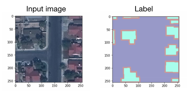
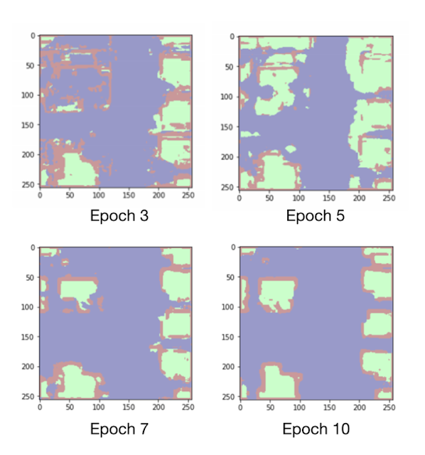
The sample code contains a walkthrough of carrying out the training and evaluation pipeline on a DLVM. The following segmentation results are produced by the model at various epochs during training for the input image and label pair shown above. This image features buildings with roofs of different colors, roads, pavements, trees and yards. We observe that initially the network learns to identify edges of building blocks and buildings with red roofs (different from the color of roads), followed by buildings of all roof colors after epoch 5. After epoch 7, the network has learnt that building pixels are enclosed by border pixels, separating them from road pixels. After epoch 10, smaller, noisy clusters of building pixels begin to disappear as the shape of buildings becomes more defined.

A final step is to produce the polygons by assigning all pixels predicted to be building boundary as background to isolate blobs of building pixels. Blobs of connected building pixels are then described in polygon format, subject to a minimum polygon area threshold, a parameter you can tune to reduce false positive proposals.

Training and model parameters

There are a number of parameters for the training process, the model architecture and the polygonization step that you can tune. We chose a learning rate of 0.0005 for the Adam optimizer (default settings for other parameters) and a batch size of 10 chips, which worked reasonably well.

Another parameter unrelated to the CNN part of the procedure is the minimum polygon area threshold below which blobs of building pixels are discarded. Increasing this threshold from 0 to 300 squared pixels causes the false positive count to decrease rapidly as noisy false segments are excluded. The optimum threshold is about 200 squared pixels.

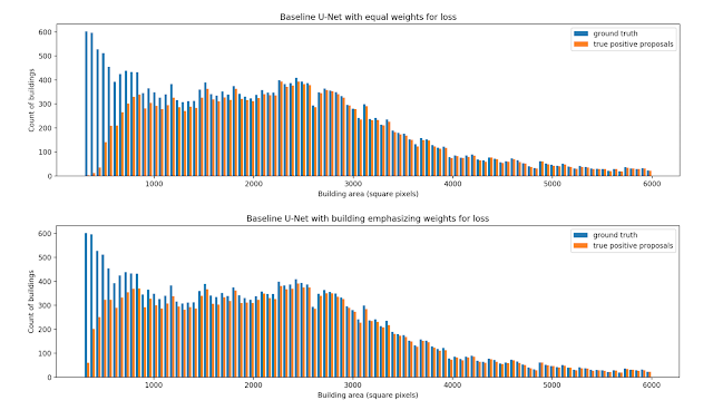
The weight for the three classes (background, boundary of building, interior of building) in computing the total loss during training is another parameter to experiment with. It was found that giving more weights to interior of building helps the model detect significantly more small buildings (result see figure below).

Each plot in the figure is a histogram of building polygons in the validation set by area, from 300 square pixels to 6000. The count of true positive detections in orange is based on the area of the ground truth polygon to which the proposed polygon was matched. The top histogram is for weights in ratio 1:1:1 in the loss function for background : building interior : building boundary; the bottom histogram is for weights in ratio 1:8:1. We can see that towards the left of the histogram where small buildings are represented, the bars for true positive proposals in orange are much taller in the bottom plot.

Last thoughts

Building footprint information generated this way could be used to document the spatial distribution of settlements, allowing researchers to quantify trends in urbanization and perhaps the developmental impact of climate change such as climate migration. The techniques here can be applied in many different situations and we hope this concrete example serves as a guide to tackling your specific problem.

Another piece of good news for those dealing with geospatial data is that Azure already offers a Geo Artificial Intelligence Data Science Virtual Machine (Geo-DSVM), equipped with ESRI’s ArcGIS Pro Geographic Information System. We also created a tutorial on how to use the Geo-DSVM for training deep learning models and integrating them with ArcGIS Pro to help you get started.

Finally, if your organization is working on solutions to address environmental challenges using data and machine learning, we encourage you to apply for an AI for Earth grant so that you can be better supported in leveraging Azure resources and become a part of this purposeful community.